Mastering Book Summarization with LLMs

Introduction

In the realm of technical prowess, utilizing Large Language Models (LLMs) to distill complete books into concise summaries stands as a remarkable feat. This endeavor reveals essential focal points:

• Complex Compression: Condensing extensive information while preserving the book’s essence.
• Strategic Abstraction: Balancing essential concepts and omitting less vital details for coherent summaries.
• Contextual Cohesion: Seamlessly weaving details into a unified narrative.
• LLM Potential: Leveraging LLMs’ linguistic prowess for effective summarization.
• Customization: Precisely tuning LLMs to fit stylistic and content preferences.

In the following sections, we will delve into the practical implementation of leveraging Large Language Models (LLMs) to perform book summarization. Our goal is to demonstrate a step-by-step approach using Python within a Jupyter notebook environment.

1. Installing Dependencies

PDF handling (PyMuPDF), core LangChain components, OpenAI integration, data manipulation (pandas, numpy), machine learning (scikit-learn), and plotting (matplotlib, plotly).

!pip install PyMuPDF langchain langchain-community langchain-openai scikit-learn python-dotenv plotly openai matplotlib pandas --quiet

2. Importing Libraries and Initial Setup

Here, we import the required libraries for numerical operations, environment variable management, plotting, clustering, dimensionality reduction, and LangChain/OpenAI functionalities. We also load environment variables (like API keys) and suppress potential future warnings for cleaner output.

import numpy as np
from dotenv import load_dotenv
import matplotlib.pyplot as plt
import fitz  # PyMuPDF for PDF processing
from openai import OpenAI # Direct OpenAI client for embeddings

# Scikit-learn components for clustering and evaluation
from sklearn.cluster import KMeans
from sklearn.metrics import silhouette_score
from sklearn.manifold import TSNE

# LangChain components for prompts, schemas, models, and text splitting
from langchain_core.prompts import PromptTemplate
from langchain_core.documents import Document
from langchain_openai import ChatOpenAI
from langchain.text_splitter import RecursiveCharacterTextSplitter
from langchain.chains.summarize import load_summarize_chain

# Load environment variables from a .env file (e.g., OPENAI_API_KEY)
load_dotenv()

# Taking out the warnings for cleaner output
from warnings import simplefilter
simplefilter(action='ignore', category=FutureWarning)

3. Loading and Extracting Text from PDF

This section focuses on opening the specified PDF file using PyMuPDF (fitz), iterating through each page to extract its text content, and then joining the text from all pages into a single string. A form feed character (chr(12)) is used here as a page separator.

# Path to your local PDF file
local_pdf_path = "Think Again - Adam Grant.pdf" # Replace with your PDF file path

# Open the PDF file using PyMuPDF
pdf_document = fitz.open(local_pdf_path)

extracted_texts = []
# Iterate through each page of the PDF
for page_num in range(pdf_document.page_count):
    page = pdf_document[page_num]
    # Extract text from the current page
    extracted_texts.append(page.get_text())

# Join the extracted text from all pages, using form feed as a separator
book_content = chr(12).join(extracted_texts)

# Close the PDF document to free up resources
pdf_document.close()

print(f"Successfully extracted text from {local_pdf_path}")

Successfully extracted text from Think Again - Adam Grant.pdf

4. Splitting Text into Manageable Chunks

The entire book content is too large to be processed by the LLM at once. We use LangChain’s RecursiveCharacterTextSplitter to divide the text into smaller, overlapping chunks based on specified separators (paragraphs, lines, tabs).

# Initialize the text splitter
text_splitter = RecursiveCharacterTextSplitter(
    separators=["\n\n", "\n", "\t"], # Define separators to split on
    chunk_size=2000,                 # Maximum size of each chunk
    chunk_overlap=200                # Overlap between consecutive chunks
)

# Split the book content into Document objects
docs = text_splitter.create_documents([book_content])

print (f"Our book is split up into {len(docs)} documents (chunks)")

Our book is split up into 315 documents (chunks)

5. Generating Embeddings for Text Chunks

To understand the semantic meaning and relationships between text chunks, we convert each chunk into a numerical vector representation called an embedding using OpenAI’s text-embedding-3-small model. We process the chunks in batches to manage API calls efficiently.

# Initialize the OpenAI client (assumes OPENAI_API_KEY is in environment variables)
client = OpenAI()

# Prepare a list of the text content from each Document object
all_texts = [doc.page_content for doc in docs]

# Set batch size for processing embeddings
batch_size = 100
vectors = [] # List to store the generated embeddings

print(f"Generating embeddings for {len(all_texts)} documents in batches of {batch_size}...")

# Process documents in batches
for i in range(0, len(all_texts), batch_size):
    # Get the current batch of text chunks
    batch_texts = all_texts[i:i+batch_size]

    # Call the OpenAI API to create embeddings for the batch
    response = client.embeddings.create(
        input=batch_texts,
        model="text-embedding-3-small" # Specify the embedding model
    )

    # Extract the embedding vectors from the API response
    batch_vectors = [item.embedding for item in response.data]

    # Add the batch embeddings to the main list
    vectors.extend(batch_vectors)

    # Optional: print progress
    print(f"Processed batch {i//batch_size + 1}/{(len(all_texts) + batch_size - 1)//batch_size}")

# Convert the list of vectors to a NumPy array for numerical operations
vectors_array = np.array(vectors)

print(f"Total embeddings generated: {len(vectors)}")
print(f"Shape of embeddings array: {vectors_array.shape}")

Generating embeddings for 315 documents in batches of 100...
Processed batch 1/4
Processed batch 2/4
Processed batch 3/4
Processed batch 4/4
Total embeddings generated: 315
Shape of embeddings array: (315, 1536)

6. Determining the Optimal Number of Clusters (Silhouette Analysis)

Before clustering, we need to determine a suitable number of clusters (k). We use the silhouette score, which measures how similar an object is to its own cluster compared to other clusters. We calculate this score for a range of k values.

# Define the range of cluster numbers to test
cluster_range = list(range(10, 30))
silhouette_avg = [] # List to store silhouette scores

print("Calculating silhouette scores for different numbers of clusters (k)...")

# Iterate through the potential number of clusters
for num_clusters in cluster_range:
    # Initialize KMeans with current k value
    kmeans = KMeans(n_clusters=num_clusters, init="k-means++", n_init=10, random_state=42)
    # Fit KMeans and predict cluster labels
    cluster_labels = kmeans.fit_predict(vectors_array)
    # Calculate the silhouette score
    score = silhouette_score(vectors_array, cluster_labels)
    silhouette_avg.append(score)
    print(f"Silhouette score for k={num_clusters}: {score:.4f}")

Calculating silhouette scores for different numbers of clusters (k)...
Silhouette score for k=10: 0.0666
Silhouette score for k=11: 0.0728
Silhouette score for k=12: 0.0770
Silhouette score for k=13: 0.0877
Silhouette score for k=14: 0.0832
Silhouette score for k=15: 0.0846
Silhouette score for k=16: 0.0930
Silhouette score for k=17: 0.0937
Silhouette score for k=18: 0.0884
Silhouette score for k=19: 0.0946
Silhouette score for k=20: 0.0913
Silhouette score for k=21: 0.0872
Silhouette score for k=22: 0.0925
Silhouette score for k=23: 0.0876
Silhouette score for k=24: 0.0982
Silhouette score for k=25: 0.0950
Silhouette score for k=26: 0.0889
Silhouette score for k=27: 0.0925
Silhouette score for k=28: 0.0867
Silhouette score for k=29: 0.0966

7. Visualizing Silhouette Scores and Selecting Optimal k

We plot the silhouette scores calculated in the previous step against the number of clusters (k). The value of k corresponding to the highest silhouette score is often considered a good choice for the number of clusters.

# Determine the optimal number of clusters based on the highest silhouette score
optimal_k_index = np.argmax(silhouette_avg)
optimal_k = cluster_range[optimal_k_index]
print(f"Optimal number of clusters (k) found: {optimal_k}")

# Plot the silhouette scores with a smaller figure size
plt.figure(figsize=(6, 4))  # Reduced from (10, 6) to (6, 4)
plt.plot(cluster_range, silhouette_avg, 'bx-')
plt.xlabel('Number of Clusters (k)')
plt.ylabel('Silhouette Score')
plt.title('Silhouette Analysis For Optimal k')
plt.xticks(cluster_range, rotation=45)  # Added rotation for better readability
plt.grid(True)
# Highlight the optimal k value
plt.scatter(optimal_k, silhouette_avg[optimal_k_index], c='red', s=80, label=f'Optimal k = {optimal_k}')  # Reduced marker size from 100 to 80
plt.legend()
plt.tight_layout()  # Added tight_layout for better spacing
plt.show()

Optimal number of clusters (k) found: 24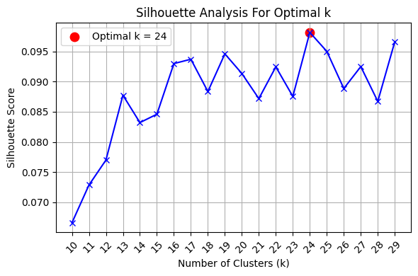

8. Performing K-means Clustering

Now, we apply K-means clustering to the embeddings using the optimal number of clusters determined from the silhouette analysis. This groups the text chunks into clusters based on their semantic similarity.

# Perform K-means clustering with the optimal number of clusters
print(f"Performing K-means clustering with k={optimal_k}...")
kmeans = KMeans(n_clusters=optimal_k, init="k-means++", n_init=10, random_state=42)
kmeans.fit(vectors_array)
# The cluster assignments for each document are stored in kmeans.labels_
print("Clustering complete.")

Performing K-means clustering with k=24...
Clustering complete.

9. Visualizing Clusters with t-SNE (3D)

To visualize the high-dimensional embeddings and their cluster assignments, we use t-SNE (t-distributed Stochastic Neighbor Embedding) to reduce the dimensionality to 3D, then create an interactive scatter plot using Plotly.

# Reduce dimensionality to 3 components using t-SNE
print("Reducing dimensions using t-SNE (3D)...")
tsne_3d = TSNE(n_components=3, random_state=42, perplexity=30, n_iter=300) # Adjust perplexity/n_iter if needed
reduced_data_tsne_3d = tsne_3d.fit_transform(vectors_array)

print("Creating 3D scatter plot...")
# Create an interactive 3D scatter plot using Plotly Express
fig_3d = px.scatter_3d(
    x=reduced_data_tsne_3d[:, 0],
    y=reduced_data_tsne_3d[:, 1],
    z=reduced_data_tsne_3d[:, 2],
    color=kmeans.labels_.astype(str), # Use cluster labels for color, converting to string for discrete colors
    title='Book Embeddings Clustered (3D t-SNE)',
    labels={'color': 'Cluster'}, # Label for the color legend
    width=800,
    height=700
)
fig_3d.update_traces(marker=dict(size=3)) # Adjust marker size if needed
# Show the plot
fig_3d.show()

Reducing dimensions using t-SNE (3D)...
Creating 3D scatter plot...

10. Visualizing Clusters with t-SNE (2D)

Alternatively, we can visualize the clusters in 2D using t-SNE and Matplotlib for a static plot.

# Reduce dimensionality to 2 components using t-SNE
print("Reducing dimensions using t-SNE (2D)...")
tsne_2d = TSNE(n_components=2, random_state=42, perplexity=30, n_iter=300)
reduced_data_tsne_2d = tsne_2d.fit_transform(vectors_array)

print("Creating 2D scatter plot...")
# Create a more compact figure
plt.figure(figsize=(10, 7))

# Plot with smaller point size
scatter = plt.scatter(reduced_data_tsne_2d[:, 0], reduced_data_tsne_2d[:, 1], 
                     c=kmeans.labels_, cmap='viridis', 
                     s=30, alpha=0.8)  # Smaller point size

plt.xlabel('t-SNE Dimension 1', fontsize=10)
plt.ylabel('t-SNE Dimension 2', fontsize=10)
plt.title('Book Embeddings Clustered (2D t-SNE)', fontsize=12)
plt.grid(True, linestyle='--', alpha=0.6, linewidth=0.5)  # Lighter grid

# Create a more compact legend that shows all clusters
all_clusters = range(optimal_k)
cmap = plt.cm.viridis
norm = plt.Normalize(vmin=0, vmax=optimal_k-1)

# Create legend handles with smaller markers
legend_handles = [plt.Line2D([0], [0], marker='o', color='w', 
                            markerfacecolor=cmap(norm(i)), 
                            markersize=8, label=f'{i}') 
                 for i in all_clusters]

# Use a multi-column legend to save space
# Calculate a reasonable number of columns based on cluster count
ncols = min(4, optimal_k // 6 + 1)  # Up to 4 columns, depending on cluster count
                                   # Adjust the divisor (6) as needed

plt.legend(handles=legend_handles, 
          title="Clusters",
          loc='best',  # Let matplotlib choose the best location
          fontsize=8,  # Smaller font size
          title_fontsize=9,
          markerscale=0.8,  # Slightly smaller markers in legend
          ncol=ncols,  # Multiple columns
          framealpha=0.7,
          handletextpad=0.3)  # Less space between marker and text

# Tight layout to minimize white space
plt.tight_layout()

plt.show()

Reducing dimensions using t-SNE (2D)...
Creating 2D scatter plot...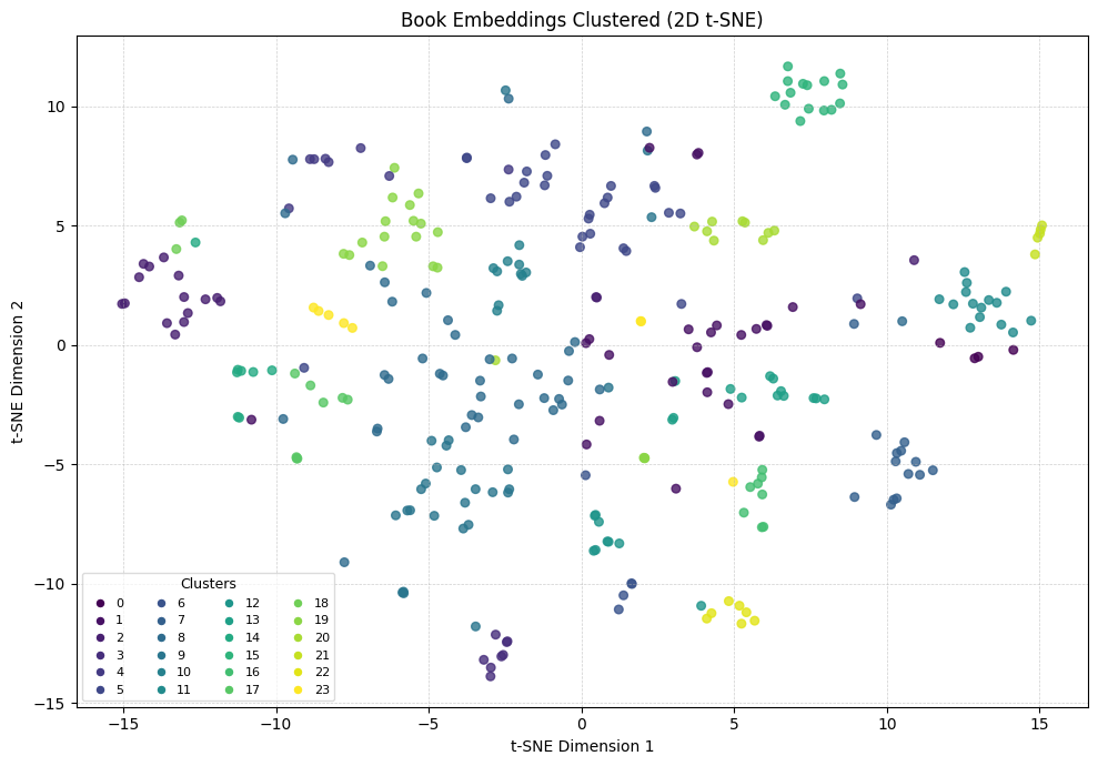

11. Selecting Representative Documents from Clusters

Instead of summarizing all chunks, we select one representative document from each cluster. We choose the document whose embedding is closest to the centroid (center) of its assigned cluster.

# Find the closest embeddings (documents) to the cluster centroids
closest_indices = []

# Loop through each cluster number (0 to optimal_k-1)
for i in range(optimal_k):
    # Get the centroid of the current cluster
    centroid = kmeans.cluster_centers_[i]
    # Calculate the Euclidean distances from the centroid to all embeddings
    distances = np.linalg.norm(vectors_array - centroid, axis=1)
    # Find the index of the document with the minimum distance
    closest_index = int(np.argmin(distances))  # Convert numpy int64 to Python int
    closest_indices.append(closest_index)

# Sort the indices for potentially ordered processing later
selected_indices = sorted(closest_indices)

print(f"Selected indices of documents closest to cluster centroids: {selected_indices}")

Selected indices of documents closest to cluster centroids: [7, 12, 27, 37, 61, 76, 80, 94, 104, 115, 133, 136, 154, 165, 170, 176, 199, 219, 248, 255, 258, 277, 288, 306]

12. Setting Up the Initial Summarization Chain (Map Step)

We define a prompt template instructing the LLM to summarize a single passage thoroughly. We then use LangChain’s load_summarize_chain with the stuff chain type (suitable for single, relatively small inputs) to create a summarization chain for individual chunks. This is the “Map” part of a potential MapReduce strategy.

# Define the prompt template for summarizing individual chunks
map_prompt = """
You will be given a single passage from a book. This section will be enclosed in triple backticks (```).
Your goal is to provide a comprehensive summary of this section, ensuring a reader understands its main points and context.
The summary should be detailed, ideally spanning multiple paragraphs to fully capture the essence of the passage.

```{text}```

FULL SUMMARY:
"""
map_prompt_template = PromptTemplate(template=map_prompt, input_variables=["text"])

# Initialize the ChatOpenAI model
llm = ChatOpenAI(temperature=0, model='gpt-4o-mini') # Use a capable and efficient model

# Load the summarization chain (stuff type for individual docs)
map_chain = load_summarize_chain(llm=llm, chain_type="stuff", prompt=map_prompt_template)
print("Map chain for individual chunk summarization is set up.")

Map chain for individual chunk summarization is set up.

13. Generating Summaries for Selected Documents

Now, we iterate through the selected document chunks (those closest to cluster centroids) and use the map_chain defined previously to generate a summary for each one.

# Get the actual Document objects corresponding to the selected indices
selected_docs = [docs[i] for i in selected_indices]

# List to hold the summaries of the selected chunks
summary_list = []

print(f"Generating summaries for the {len(selected_docs)} selected documents...")

# Loop through the selected documents
for i, doc in enumerate(selected_docs):
    print(f"Summarizing document {i+1}/{len(selected_docs)} (original index {selected_indices[i]})...")
    # Run the map_chain to get the summary for the current document chunk
    # Note: 'stuff' chain expects a list, even if it's just one document
    chunk_summary = map_chain.run([doc])
    # Append the generated summary to the list
    summary_list.append(chunk_summary)
    # Optional: print a snippet of the summary
    # print(f"  Summary snippet: {chunk_summary[:100]}...")

print("Finished generating individual summaries.")

Generating summaries for the 24 selected documents...
Summarizing document 1/24 (original index 7)...
Summarizing document 2/24 (original index 12)...
Summarizing document 3/24 (original index 27)...
Summarizing document 4/24 (original index 37)...
Summarizing document 5/24 (original index 61)...
Summarizing document 6/24 (original index 76)...
Summarizing document 7/24 (original index 80)...
Summarizing document 8/24 (original index 94)...
Summarizing document 9/24 (original index 104)...
Summarizing document 10/24 (original index 115)...
Summarizing document 11/24 (original index 133)...
Summarizing document 12/24 (original index 136)...
Summarizing document 13/24 (original index 154)...
Summarizing document 14/24 (original index 165)...
Summarizing document 15/24 (original index 170)...
Summarizing document 16/24 (original index 176)...
Summarizing document 17/24 (original index 199)...
Summarizing document 18/24 (original index 219)...
Summarizing document 19/24 (original index 248)...
Summarizing document 20/24 (original index 255)...
Summarizing document 21/24 (original index 258)...
Summarizing document 22/24 (original index 277)...
Summarizing document 23/24 (original index 288)...
Summarizing document 24/24 (original index 306)...
Finished generating individual summaries.

14. Combining Individual Summaries

The individual summaries generated in the previous step are combined into a single text block, separated by newlines. We convert this combined text back into a LangChain Document object, ready for the final summarization step. We also check the token count.

# Join the individual summaries into one large string
summaries_combined = "\n\n---\n\n".join(summary_list) # Use a clear separator

# Convert the combined summaries string into a single Document object
summaries_doc = Document(page_content=summaries_combined)

print("Combined individual summaries into a single document.")
# Calculate and print the total number of tokens in the combined summary document
total_tokens = llm.get_num_tokens(summaries_doc.page_content)
print(f"The combined summary document has approximately {total_tokens} tokens.")

Combined individual summaries into a single document.
The combined summary document has approximately 8999 tokens.

15. Generating the Final Combined Summary (Reduce Step)

Finally, we define a “combine” prompt instructing the LLM to synthesize the collection of chunk summaries into a single, cohesive, and verbose summary of the entire book. We use another load_summarize_chain (again, stuff type is often sufficient if the combined summaries aren’t excessively long) to perform this final reduction and generate the end result.

# Define the prompt template for combining the summaries
combine_prompt = """
You will receive a series of summaries representing different sections of a book, separated by '---'. These summaries are enclosed in triple backticks (```).
Your task is to synthesize these summaries into a comprehensive overview of the entire book.
The final summary should be detailed and allow a reader to grasp the main arguments, narrative, and key takeaways of the book.
Structure the final summary logically, using bullet points for key themes or chapter-like sections where appropriate.

```
{text}
```

COMPREHENSIVE BOOK SUMMARY:
"""
combine_prompt_template = PromptTemplate(template=combine_prompt, input_variables=["text"])

# Load the summarization chain for the final combination step
# Using 'stuff' chain again, assuming the combined summaries fit context window.
# If 'total_tokens' is very large, consider 'map_reduce' or 'refine' chain types.
reduce_chain = load_summarize_chain(llm=llm, chain_type="stuff", prompt=combine_prompt_template)

print("Generating the final comprehensive summary...")
# Run the reduce_chain on the combined summary document
final_output = reduce_chain.run([summaries_doc])

# Print the final book summary
from IPython.display import Markdown, display
display(Markdown("# Final Book Summary: *Think Again* by Adam Grant\n\n" + final_output))

Generating the final comprehensive summary...

Final Book Summary: Think Again by Adam Grant

The book presents a multifaceted exploration of the concept of “rethinking,” emphasizing its critical role in personal growth, interpersonal influence, and community development. Through a series of narratives, case studies, and psychological insights, the author illustrates how adaptability and open-mindedness can lead to better decision-making and improved outcomes in various contexts. Below is a comprehensive overview of the book’s key themes and arguments:

1. The Importance of Rethinking

• Definition and Relevance: Rethinking is framed as the ability to question and amend one’s beliefs and mental frameworks, akin to how the U.S. Constitution can be amended. This flexibility is essential for navigating complex and rapidly changing environments.
• Personal Cognitive Flexibility: The author shares stories of individuals who have successfully navigated their mental barriers, such as a Nobel Prize-winning scientist who values being wrong and an entrepreneur who overcomes outdated beliefs.

2. The Struggle Between Instinct and Training

• Case Study of Mann Gulch: The narrative of smokejumpers during a wildfire illustrates the tension between survival instincts and professional training. The crew’s reluctance to abandon their heavy equipment led to tragic consequences, highlighting the need for adaptability in high-stakes situations.
• Lessons from Other Disasters: The author references other incidents, such as the Storm King Mountain fire, to reinforce the idea that rigid adherence to training can be detrimental.

3. Influencing Others’ Thinking

• Effective Persuasion: The book discusses various examples of individuals who have successfully influenced others, such as a musician who changes the views of white supremacists and a doctor who alters parents’ perceptions about vaccines through empathetic communication.
• Constructive Conflict: The author emphasizes the value of open disagreement in creative processes, using examples from filmmakers and the Wright brothers to illustrate how passionate debates can lead to innovation.

4. The Dunning-Kruger Effect and Overconfidence

• Understanding Limitations: The book explores the Dunning-Kruger effect through the story of Iceland’s former central bank governor, illustrating how overconfidence can lead to poor decision-making and a lack of awareness of one’s limitations.
• Metacognitive Skills: The importance of self-reflection and the ability to assess one’s own knowledge is highlighted as crucial for personal and professional growth.

5. The Role of Emotional Engagement in Communication

• Forecasting and Emotional Biases: The author discusses how emotional biases can cloud judgment in political forecasting, emphasizing the need to detach personal identity from predictions to improve accuracy.
• Perspective-Seeking: The book advocates for engaging in meaningful conversations to understand differing viewpoints, suggesting that emotional engagement can enhance trust and respect in discussions.

6. The Challenges of Traditional Education

• Critique of Lecturing: The author critiques the reliance on traditional lecturing in education, arguing that it often fails to foster critical thinking and active learning among students.
• Innovative Teaching Methods: The narrative introduces Ron Berger’s hands-on teaching approach, which emphasizes problem-solving and iterative learning, encouraging students to engage deeply with material.

7. Psychological Safety in Organizations

• Creating Safe Environments: The book discusses the importance of psychological safety in fostering open communication within teams, drawing parallels to historical events like the Challenger disaster to illustrate the consequences of failing to address concerns.
• Long-term Benefits: The author emphasizes that cultivating psychological safety can lead to improved team dynamics and innovation.

8. Navigating Career Paths and Personal Growth

• Self-Reflection and Career Checkups: The author encourages individuals to regularly assess their career aspirations and align them with personal growth, using anecdotes to illustrate the importance of adaptability in career choices.
• Life Checkups: The concept of scheduling regular evaluations of one’s life trajectory is presented as a proactive approach to ensure alignment with personal values and goals.

9. The Power of Listening and Empathy

• Empathetic Engagement: The book highlights the transformative power of listening, as illustrated by the character Betty, who fosters understanding in conflict-ridden environments through patient listening and engagement.
• Motivational Interviewing: The author discusses the principles of motivational interviewing, emphasizing the need for genuine communication to guide others toward change.

10. Addressing Climate Change Denial

• Communication Challenges: The author explores the complexities of climate change denial and the importance of nuanced communication strategies that resonate with diverse audiences.
• Incorporating Values: The book suggests that effective messaging should appeal to a broader range of values, including conservative ideals, to engage skeptics in climate action.

Conclusion

The book serves as a comprehensive guide to the art of rethinking, emphasizing the necessity of adaptability, open-mindedness, and effective communication in personal and professional contexts. Through a blend of narratives, psychological insights, and practical strategies, the author encourages readers to embrace the discomfort of questioning their assumptions and to view rethinking as a pathway to growth and understanding.